LLM inference: core concepts and terms
LLM inference is a pipeline. The server receives requests and groups them into batches. It reads each prompt in one pass, which is called prefill. Then it makes the output one token at a time, which is called decode. This post collects the abbreviations and feature names that attach to each part of this pipeline.
Almost every term serves one of two goals: keep the GPU busy, or get the answer to the user sooner. With these two goals in mind, each new term is easier to place.
About this post
This post is based on the Zhihu article 大模型推理核心概念与术语总结 (“Key concepts and terms of large model inference”) by kaiyuan, from the InfraTech series. I put the terms in a new order, added worked examples, and marked the places where the article is unclear or differs from common usage. In this post, “the source article” means that article. All figures are new drawings.
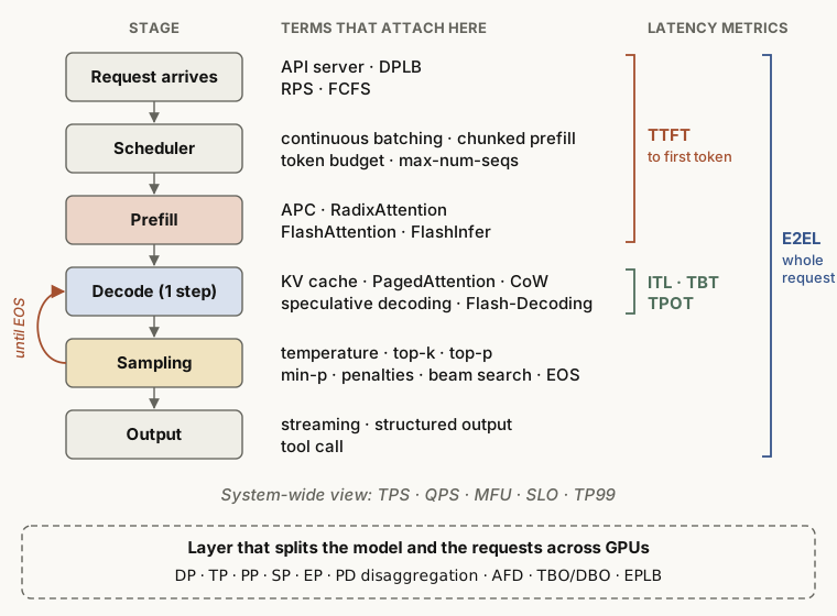
Two stages to know first: prefill and decode
The source article starts with a list of terms. But almost every term targets one of two stages, so this post explains these stages first.
- Prefill (prompt processing)
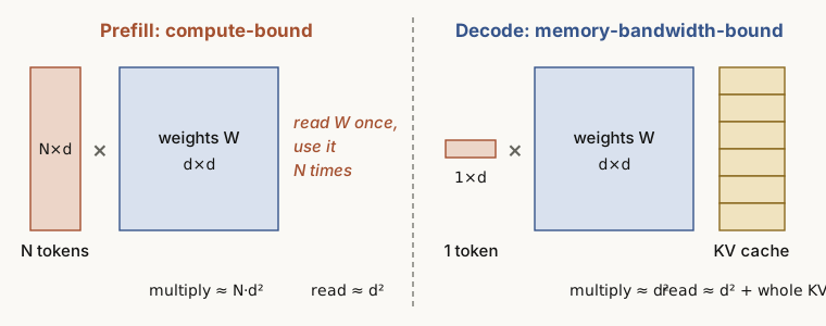
- The model runs the full prompt through all layers in one pass and makes the first output token. It computes N tokens at the same time, so the GPU compute units stay full. Prefill is compute-bound.
- Decode (generation)
- After prefill, the model makes one new token per step. Each step computes only one token, but it must read all the model weights and the full KV cache from memory. Decode is memory-bandwidth-bound. The source article calls it “storage-bound”.
- KV cache (key-value cache)
- The memory that keeps the key and value vectors of the tokens that attention already processed. Without it, the model must compute all the earlier text again for each new token.
Analogy
Prefill is like a student who reads the whole exam paper once at the start. Decode is like a student who writes the answer one letter at a time. Before each letter, the student opens the full textbook (the weights) and the answer so far (the KV cache) again. Most of the time goes to reading, so the hand that writes (the compute units) often waits.
In short
Prefill runs out of compute first, and decode runs out of memory bandwidth first. Most techniques in this post answer one question: how do we mix or separate these two bottlenecks so that the GPU does not sit idle?
Core features: what an engine offers
The source article lists about 20 features of inference engines such as vLLM and SGLang. This post puts related features into groups.
Batching: keep the GPU busy
- Continuous batching (iteration-level batching)
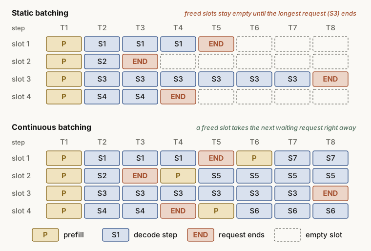
- The engine does not run a fixed batch to the end. At each decode step, it removes the finished requests and adds new requests at once. This is the most basic way to keep the GPU busy.
Static batching waits until the longest request in the batch is done. When a short request ends early, its slot stays empty. Continuous batching gives that slot to a waiting request at once.
Analogy
Static batching is like a four-seat ride that waits until all four riders get off before it takes new riders. Continuous batching gives a free seat to the next person in line as soon as one rider gets off.
KV cache memory management
- PagedAttention
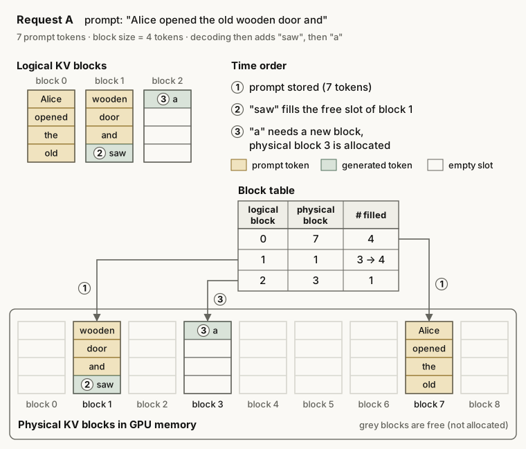
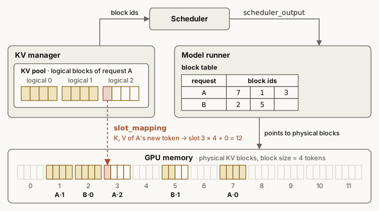
- The engine divides the KV cache into blocks of fixed size, for example 16 tokens per block. A block table maps the logical blocks of each request to physical blocks in GPU memory. The idea is the same as virtual memory paging in an operating system, and it reduces memory fragmentation.
- Copy-on-write (CoW)
- Several requests can share the blocks of a common prefix. The engine copies a shared block only when one request must write different content into it. Until that write, no block is copied.
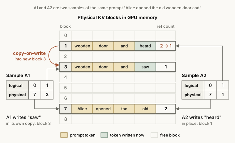
- RadixAttention (SGLang)
- SGLang keeps the token sequences of requests in a radix tree, so requests with the same prefix share their KV cache automatically. The KV tensors sit in non-contiguous pages, and by default one page holds one token (
--page-size 1). When memory is full, SGLang evicts leaf nodes, by default with an LRU (least recently used) policy. The source article spells the name “Radix Attetnion” by mistake.
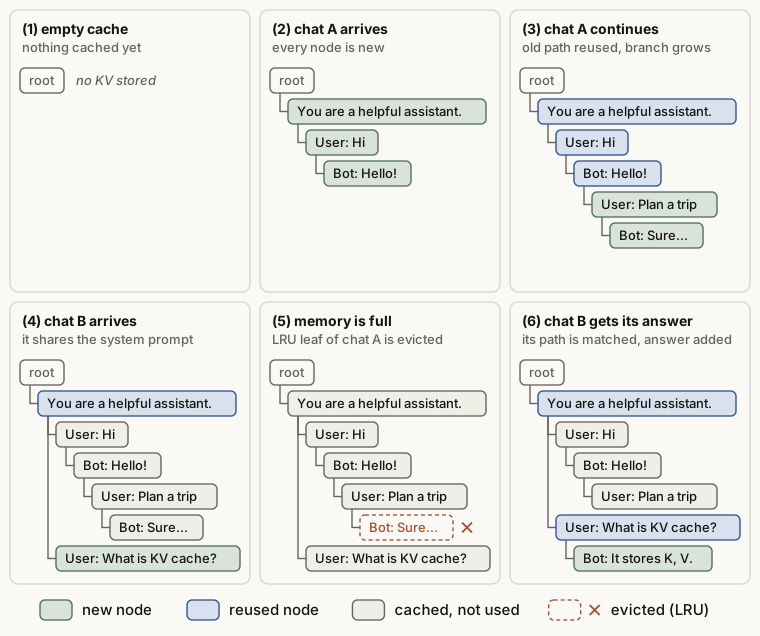
- APC (automatic prefix caching)
- A new request can start with the same prefix as an earlier request. The engine then reuses the stored KV cache for that prefix. Prefill has less to compute, so the time to first token (TTFT) goes down. APC in vLLM has the same goal as RadixAttention but uses hash-based block matching.
Disaggregation: different work on different machines
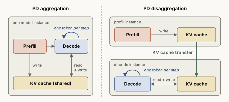
- PD disaggregation (prefill-decode disaggregation)
- The engine puts the compute-bound prefill (P) and the memory-bound decode (D) on different GPUs or instances. The prefill side makes the KV cache and sends it to the decode side, and the decode side continues the generation. The two stages no longer interrupt each other. Each side can use its own GPU count, parallelism and batch size. So the engine can tune TTFT and ITL separately, and more requests meet their latency targets on each GPU. PD disaggregation alone does not raise the raw throughput.
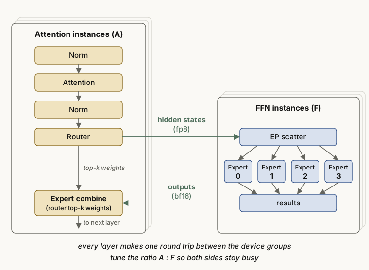
- AFD (attention-FFN disaggregation)
- AFD splits the work more finely than PD disaggregation. Inside one layer, the attention part and the FFN part (in particular the MoE experts) run on different devices. You tune the ratio of attention devices (A) to FFN devices (F) so that both sides stay busy.
Faster decode
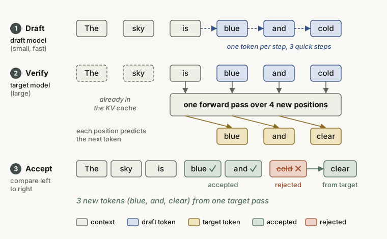
- Speculative decoding
- A small, fast draft model guesses several tokens first. The large target model then checks all the guesses in one forward pass. The engine keeps the guesses up to the first wrong one, and from that point it uses the token of the large model. This is the rule for greedy decoding. With sampling, the engine accepts each guess with the probability min(1, p/q). Here p and q are the probabilities from the large and the small model. If it rejects a guess, it samples a replacement from a corrected distribution. So the output follows the distribution of the large model exactly. This works because decode is memory-bound: the large model needs about the same time to check one token or five tokens.
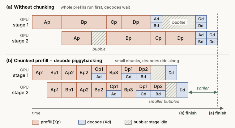
- Chunked prefill
- The engine cuts a long prefill into small chunks along the sequence. Each chunk goes into the same batch as the decode requests of that step. A long prefill can then no longer take the whole GPU and stop the decode of other requests. The chunks also use the compute that decode alone leaves idle.
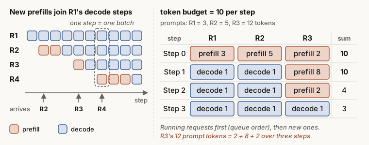
Worked example: the token budget
Check the right side of Figure 11 with numbers. The budget is 10 tokens per step. In step 0, 3 + 5 + 2 = 10. In step 1, R1 and R2 have finished prefill, so each gets one decode token. R3 has 12 − 2 = 10 prefill tokens left, and the budget allows 8 of them (1 + 1 + 8 = 10). In step 2, R3 gets its last 2 prefill tokens, plus the two decode tokens (1 + 1 + 2 = 4). From step 3, all three requests decode one token per step.
The vLLM docs describe the rule like this: put the decode tokens in first, then fill the rest of the budget with prefill chunks. The current V1 scheduler is a little different. It serves the running requests first, in queue order, and a running request can also be an unfinished prefill. New requests then use the rest of the budget. In this example, both rules give the same steps. Smaller chunks make the decode latency (ITL) more stable. But one prefill then spans more steps, so its TTFT can go up.
Quantization, LoRA and output control
- W8A16 (8-bit weights, 16-bit activations)
- The weights (W) are stored in 8 bits (INT8 or FP8), and the activations (A) keep 16-bit floating-point precision, such as FP16. Related formats are W8A8 and W4A16. Sometimes the data type follows the name, as in
w8a8_int8.
Why shrink only the weights?
In a dense model at a small batch size, decode reads all the weights at each step. So the weight size in bytes sets most of the step time. A 7B (7 billion parameter) model needs about 14 GB in FP16, at 2 bytes per parameter. In INT8 (1 byte) it needs about 7 GB, and in 4-bit about 3.5 GB. When the engine reads half the bytes, memory-bound decode can become up to twice as fast. W8A8 also makes the activations 8-bit, so the matrix multiplications can run on INT8 units. The risk of accuracy loss is higher.
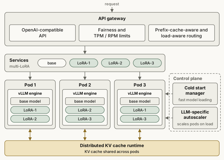
- Multi-LoRA (serving many LoRA adapters at once)
- One base model carries many small LoRA adapters, and each adapter is fine-tuned for one task. For each request, the engine selects the adapter that the request needs. All requests share the weights of the base model.
- Guided decoding
- At each step, the engine removes the tokens that would break a given format or grammar, such as JSON, SQL or a regular expression. So the output that the model has made so far is always valid. The output is complete unless generation stops early, for example at
max_tokens. The source article calls this feature “Guided Decoder”. - Function call / tool call
- The model is trained to output a function call in a fixed format, and the engine parses the call from the output. This lets the LLM call external tools. Guided decoding can also force the call to match the argument schema of the function.
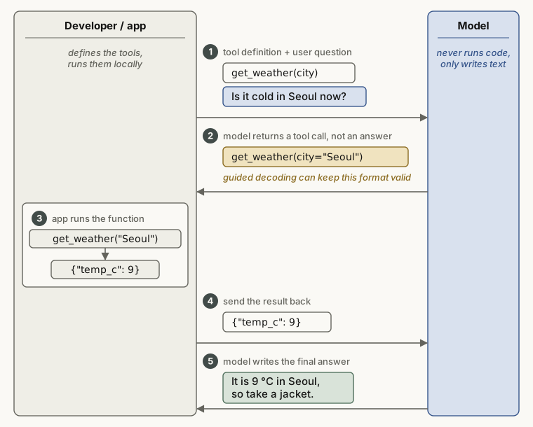
get_weather(city) and the user question to the model. (2) The model does not answer yet. It returns a call, get_weather(city="Seoul"). Guided decoding can keep this format valid (in vLLM, for a named tool or tool_choice="required"). (3) The app runs the function. (4) The app sends the result {"temp_c": 9} back to the model. (5) The model writes the final answer.Parallelism and overlap
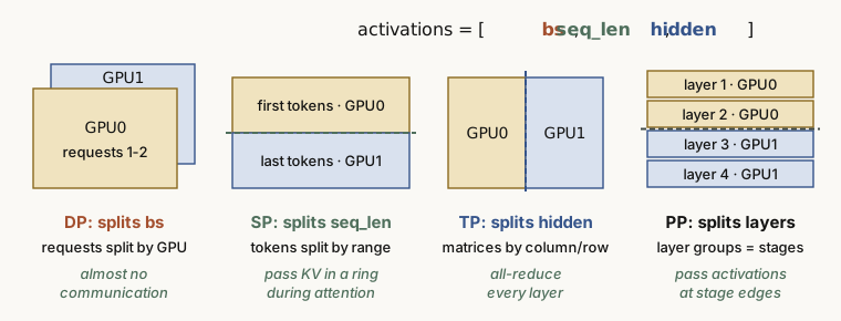
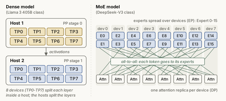
- DP / SP / TP / PP (data, sequence, tensor and pipeline parallelism)
- These are the four basic ways to split a model or its requests across GPUs. DP splits the batch of requests. SP splits the token sequence. TP splits the hidden dimension, which means the weight matrices. PP splits the layers.
A small figure in the source article maps DP, SP and TP to the three axes of the activation tensor [bs, seq_len, hidden_size]. Figure 13 adds PP to that picture.
- TBO / DBO (two-batch overlap / dual-batch overlap)
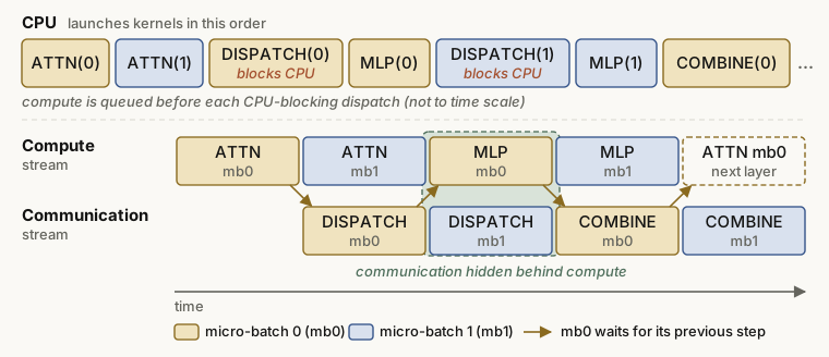
- The engine splits the requests into two micro-batches and runs them out of phase. While one micro-batch does attention, the other does the dispatch and combine communication for the experts. The compute stream and the communication stream run at the same time, so each hides the wait time of the other.
Attention kernels
- FA (FlashAttention)
- An algorithm that computes attention fast. FlashAttention-1 uses the online softmax method to fuse QKᵀ, softmax and ×V into one kernel. So it never writes the large attention matrix to HBM (the global memory of the GPU) and reads it back. FlashAttention-2 divides the work better and uses fewer operations that are not matrix multiplications. This helps on NVIDIA A100 and H100 class GPUs, where the units outside the tensor cores are slow.
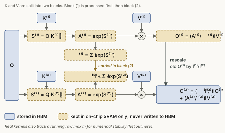
Here $l$ is the sum of the exponentials so far (the softmax denominator), and $A = \exp(S)$ is the weight before normalization. Real kernels also update the row maximum $m$ for numerical stability. The figure leaves $m$ out.
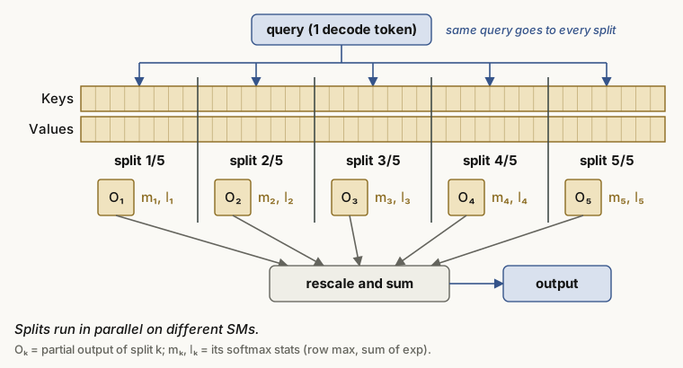
- Flash-Decoding
- In decode, the query has only one token. FlashAttention splits the work over the batch, the heads and blocks of the query. In decode the query is one token, so with a small batch and a long context, most of the GPU sits idle. Flash-Decoding splits the long KV sequence into parts instead and computes the parts in parallel. At the end, it combines the parts with a softmax correction.
- FlashInfer
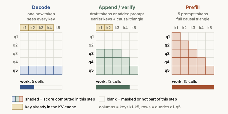
- An attention kernel library that inference frameworks use under the hood. The shapes of the query and the KV differ between inference stages, so FlashInfer has optimized FlashAttention kernels for prefill, append and decode. Append uses the same API as prefill. The source article writes “FIA (Flash Infer Attention)”, but FlashInfer itself does not use the name FIA. On Huawei Ascend NPUs, FIA means Fused Infer Attention, a fused operator that also picks a prefill or decode kernel by the query shape. The figure in the source article matches the FlashInfer material, so this post follows FlashInfer.
- Linear attention
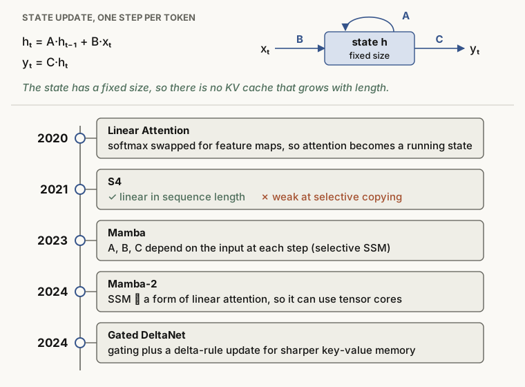
- The cost of softmax attention grows with the square of the sequence length. Linear attention models replace it with the update of a state of fixed size, so the cost grows linearly with the length. They need less memory and compute faster. The source article says that hybrid models with some linear attention layers keep getting more accurate. It adds that in some areas they reach the level of standard (full) attention.
Load balancing
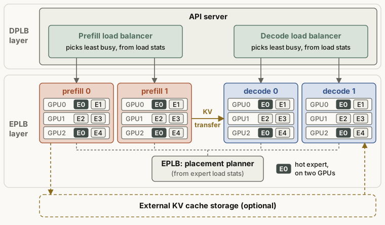
- DPLB (data-parallel load balancing)
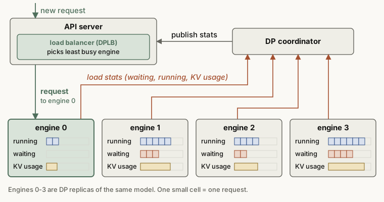
- A scheduler that spreads requests evenly over the engine instances of a DP deployment. Each engine reports its running and waiting requests. In vLLM, a coordinator collects these reports and publishes them to the API server. The API server then sends the new request to a less busy engine.
- EPLB (expert-parallelism load balancer)
- In an MoE model, many tokens can go to the same few experts. Then only the GPUs that hold those experts are busy. EPLB copies or moves the popular experts so that the load is even across devices.
The feature list of the source article also names multi-step scheduling: the engine plans several decode steps in one scheduler call, which cuts CPU overhead. The source article gives no more detail, so the name is enough for now. vLLM had this feature in its older V0 engine (--num-scheduler-steps). The current V1 engine does not have it.
Performance metrics: what to measure
Inference metrics measure the quality of a service by how fast it makes tokens. They fall into two groups. The first group is the latency that one request sees (TTFT, ITL, E2EL). The second group is the throughput of the whole system (TPS, QPS).
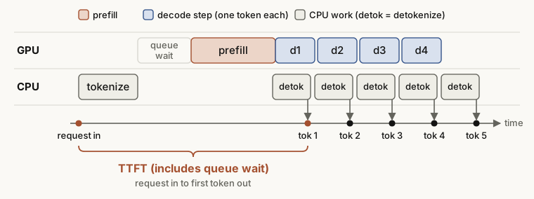
- TTFT (time to first token)
- The time from the request to the first output token. Most of it is prefill time, so TTFT is the main prefill metric.
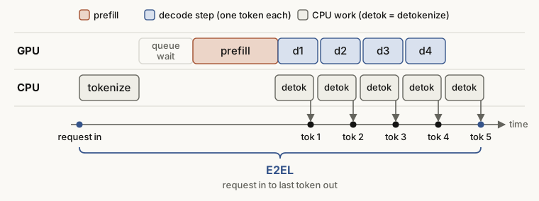
- E2EL (end-to-end latency)
- The time from the prompt input until the system returns the full result.
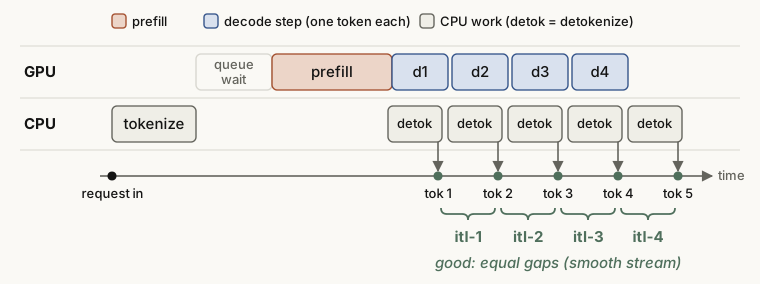
- ITL (inter-token latency)
- The (average) time to make one token in the decode stage. The common formula, from the GenAI-Perf definition, is below.
Here $n$ is the number of output tokens. TTFT already contains the first token, so the formula divides by the $n - 1$ gaps that remain.
- TBT (time between tokens)
- The time between two consecutive tokens. It usually means the time of one specific token: TBTᵢ = latencyᵢ − latencyᵢ₋₁.
- TPOT (time per output token)
- In the definition of the source article, the average time per token, with the first token included: TPOT = E2EL / n.
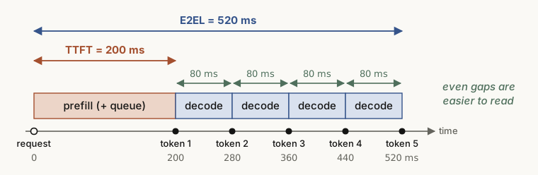
| Metric | Formula | Value in Figure 25 |
|---|---|---|
| TTFT | time of first token − time of request | 200 ms |
| E2EL | time of last token − time of request | 520 ms |
| ITL | (E2EL − TTFT) / (n − 1) | (520 − 200) / 4 = 80 ms |
| TBT₃ | latency₃ − latency₂ | 360 − 280 = 80 ms |
| TPOT (source article) | E2EL / n | 520 / 5 = 104 ms |
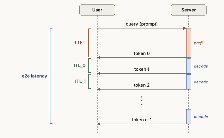
The names and formulas differ between tools
The source article notes that some tools, such as vLLM, compute ITL the way this post defines TBT: one gap per token. (More exactly,
vllm bench servemeasures one gap per streamed chunk, which is usually one token.) They compute TPOT the way this post defines ITL: (E2EL − TTFT) / (n − 1). Most benchmarks today define TPOT as the average without the first token. So it is safer to treat TPOT = E2EL / n, with the first token included, as a minority definition. In the example above, the two definitions give 104 ms and 80 ms, which is a large difference. Before you compare benchmark numbers, always check which formula they use.
Throughput and service targets
- QPS (queries per second)
- The number of requests that the system completes per second. The source article gives the formula QPS = T / Σ latency(i).
- TPS (tokens per second)
- The total number of output tokens per second: TPS = n_tokens / (T_y − T_x), in tok/s. Here T_x is the time when the first request is sent, and T_y is the time when the last response arrives.
- QPM (queries per minute)
- The number of requests that the system completes per minute.
- TP90 / TP99 (top percentile, often called P90 / P99)
- The value that 90% (or 99%) of requests meet. For example, when the TP99 of TTFT is 1 second, 99 of 100 requests got their first token within 1 second. TP50 (the median) is similar.
- RPS (requests per second)
- In a load test, the number of requests that the test sends per second. It is a main setting of a throughput test. Some tools, such as those from NVIDIA, use RPS for the requests completed per second, which is QPS in this post. Check which one a report means.
- Ramp-up test
- A test that changes the RPS step by step and records how the service performance changes.
- SLO (service level objective)
- The quality target that the service must meet. For example: “In the last period, did at least 99% of the requests get 20 tok/s or more each?” This example uses the output speed of each request (TPS per user, close to 1 / ITL for long outputs), not the system TPS above. 20 tok/s per user means an ITL of 50 ms or less.
- MFU (model FLOPs utilization)
- The fraction of the theoretical compute of the GPU that the model actually uses.
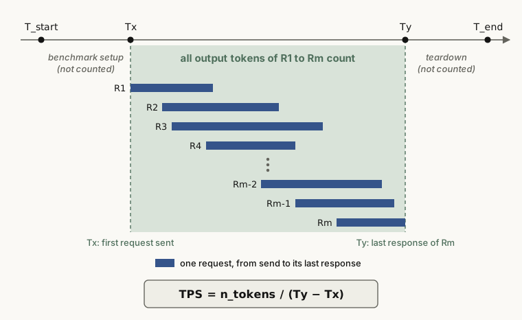
A closer look at QPS
The QPS formula of the source article is ambiguous, because T also appears in the range of the sum. A common definition in practice is the number of requests completed in the window, divided by the length of the window in seconds. A server runs many requests at the same time, so a division by the sum of latencies underestimates the throughput.
Latency and throughput also pull against each other. A larger batch raises TPS, but it also raises the ITL of each request. An SLO sets the limit in this trade-off, for example: “the highest throughput that keeps latency under this line”.
Sampling: rules for the next token
At each step, the model gives a score (a logit) for every token in the vocabulary. Sampling turns these scores into probabilities, keeps some candidates, and picks one of them. The source article puts sampling at the end of the metrics section. This post gives it a section of its own.
- Temperature
- The engine divides the logits by T and then applies softmax, which changes the shape of the whole distribution. With T < 1, the distribution becomes sharper, and the top token becomes more likely. With T > 1, it becomes flatter, and the answers vary more.
- Top-k
- Sort the tokens by probability and keep only the top k. The range is 1 to vocab_size. In vLLM, 0 (the default) or −1 turns the filter off. In Hugging Face Transformers, 0 turns it off.
- Top-p (nucleus sampling)
- Sort the probabilities from high to low as $p_{(1)} \ge p_{(2)} \ge \dots \ge p_{(V)}$. Keep the first k tokens, where k is the first point at which the cumulative sum $C_k = \sum_{i=1}^{k} p_{(i)}$ reaches P or more. P is between 0 and 1.
- Min-p
- Keep only the tokens with a probability of at least min-p times the top probability. The source article gives the range as “> 0”, but in practice the value is between 0 and 1.
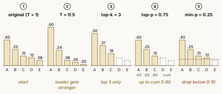
Worked example: follow the numbers
With T = 0.5: softmax(z/T) is the same as $p_i^{1/T}$ after normalization, so here the engine normalizes $p_i^2$. The squares are 0.16, 0.0625, 0.0225, 0.0144 and 0.0064, and their sum is 0.2658. After the division, they become 0.60, 0.24, 0.08, 0.05 and 0.02. So A goes from 0.40 to 0.60.
With top-k = 3, keep A, B and C and divide by their sum, 0.80. The result is 0.50, 0.31 and 0.19.
With top-p = 0.75, the cumulative sums are 0.40, 0.65 and 0.80. The engine stops at C₃ = 0.80 ≥ 0.75 and keeps three tokens. The result is the same as with top-k only by chance. Top-p is an adaptive cut: it keeps one or two tokens when the distribution is sharp, and many tokens when it is flat.
With min-p = 0.25, D has 0.12 ≥ 0.10, so D stays, and only E goes. Min-p is also adaptive, because the threshold scales with p_max. The order of these steps in real engines (penalties, then temperature, then top-k, top-p and min-p, then the sample) differs a little between implementations.
- Frequency penalty
- Lowers the logit of each token that already appeared, in proportion to the number of times it appeared. More appearances give a larger cut.
- Presence penalty
- Subtracts a fixed value from the logit of each token that appeared at least once. The cut happens once per token, whatever the count.
- Repetition penalty
- Reduces tokens that already appeared. The source article compares it to the frequency penalty. But vLLM and Hugging Face apply it once per token, whatever the count, and they also count prompt tokens. They scale the logit: they divide a positive logit by the penalty and multiply a negative one by it.
- Beam search
- At each step, the search keeps only the k candidate sequences with the highest cumulative probability (k is the beam width) and prunes the rest. You can think of it as top-k plus pruning, applied to whole sequences.
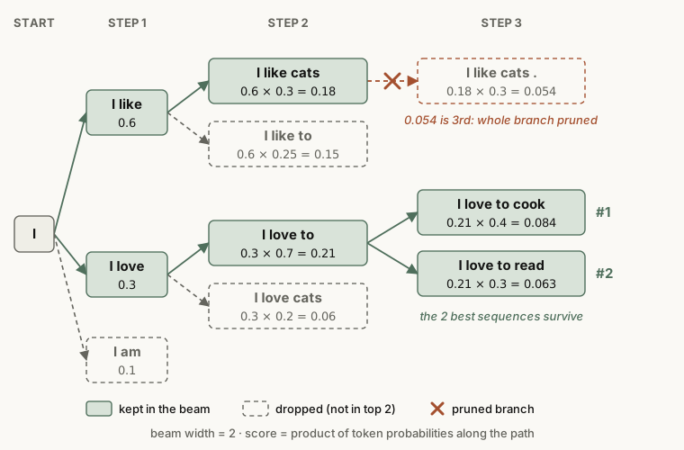
Worked example: beam search
At step 2, “I like cats” = 0.6 × 0.3 = 0.18 and “I love to” = 0.3 × 0.7 = 0.21 stay. At step 3, the best extension of “I like cats” gives 0.18 × 0.3 = 0.054. The extensions of “I love to” give “read” with 0.21 × 0.3 = 0.063 and “cook” with 0.21 × 0.4 = 0.084. The top two (0.084 and 0.063) both come from the lower branch, so the search prunes the upper branch.
A greedy search takes only the top token at each step, so it would take “like” (0.6) at step 1. Beam search finds that the “love” path wins in the end, although it was second at first. The cost is extra computation that grows with the beam width.
Engines and frameworks
- vLLM
- A widely used inference framework from the Sky Computing Lab at UC Berkeley. It started from PagedAttention. Its strengths are many features and a large ecosystem.
- SGLang
- Another main framework, from UC Berkeley and Stanford. It started from RadixAttention, and its main claim is speed.
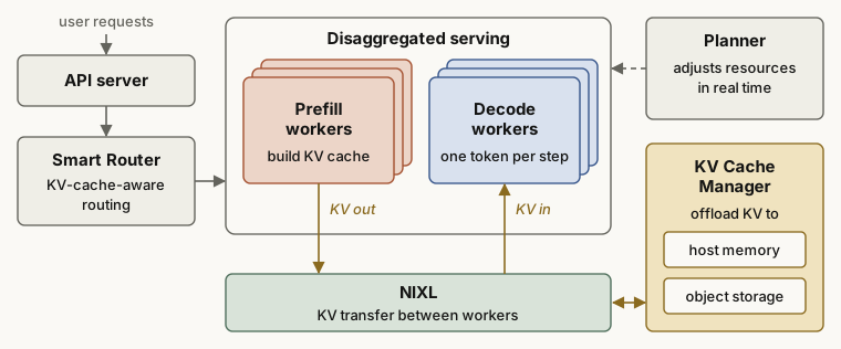
- Dynamo
- The distributed inference system of NVIDIA. It runs on top of engines such as vLLM and SGLang and adds PD disaggregation, KV-aware routing and KV offloading.
- AIBrix
- A cloud-native LLM inference solution from ByteDance, based on Kubernetes.
Main serving parameters in vLLM
| Parameter | Meaning |
|---|---|
max-num-seqs | The maximum number of sequences in one step (iteration) |
max-num-batched-tokens | The maximum number of tokens in one step. It controls the total token count (the token budget in Figure 11) |
max-model-len | The context length of the model (the maximum of input plus output tokens). If you do not set it, vLLM reads it from the model config |
max-input-length | The limit on the input length. The source article lists it, but current vLLM has no such flag; max-model-len limits the context |
load-format | The format to load the weights. "dummy" fills the weights with random values, mainly for performance analysis |
dtype | The data type of weights and activations: auto, half, float16, bfloat16, float, float32 |
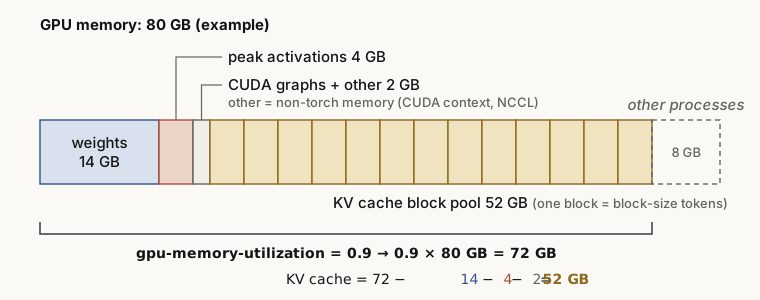
gpu-memory-utilization | The fraction of the total GPU memory that this vLLM instance can use. vLLM fills the unused part of this budget with KV cache, so the value is a budget, not the real load. |
block-size | The number of consecutive tokens in one KV cache block |
enforce-eager | Always run PyTorch in eager mode, with no CUDA graph capture |
pipeline-parallel-size (pp) | The number of pipeline stages |
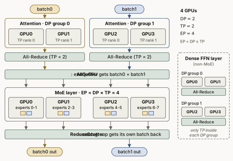
tensor-parallel-size (tp) | The tensor-parallel size: the number of GPUs that share each layer |
data-parallel-size | The number of data-parallel replicas |
enable-expert-parallel | Use expert parallelism instead of tensor parallelism for the MoE layers. EP = DP × TP |
Main serving parameters in SGLang (memory and scheduling)
The source article shows a table from the SGLang documentation as an image, in Chinese. The table below gives its content.
| Parameter | Description | Default |
|---|---|---|
mem_fraction_static | The fraction of GPU memory for static memory, such as model weights and the KV cache. Increase it if the KV cache cannot be built. Decrease it if CUDA runs out of memory | None |
max_running_requests | The maximum number of requests that run at the same time | None |
max_total_tokens | The maximum number of tokens that the KV cache can hold. Mainly for debugging | None |
chunked_prefill_size | Run prefill in chunks of this size. A larger value makes prefill faster but uses more VRAM. Decrease it if CUDA runs out of memory | None |
max_prefill_tokens | The token budget of one prefill batch. The real limit is the larger of this value and context_length | 16384 |
schedule_policy | The scheduling policy: the order in which one engine processes the waiting prefill requests | "fcfs" |
schedule_conservativeness | How cautious the engine is when it accepts new prefill requests. A high value can cause starvation, and a low value can slow down decode | 1.0 |
cpu_offload_gb | The RAM (in GB) to reserve for offloading model parameters to the CPU | 0 |
The parameters change between engine versions. Before you use them, check the official vLLM and SGLang documentation.
Main modules of the vLLM engine
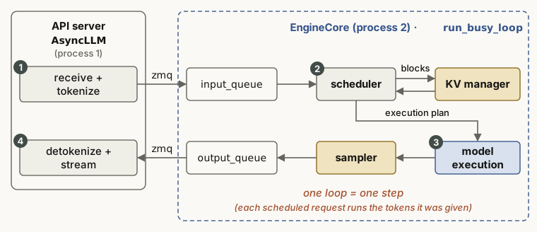
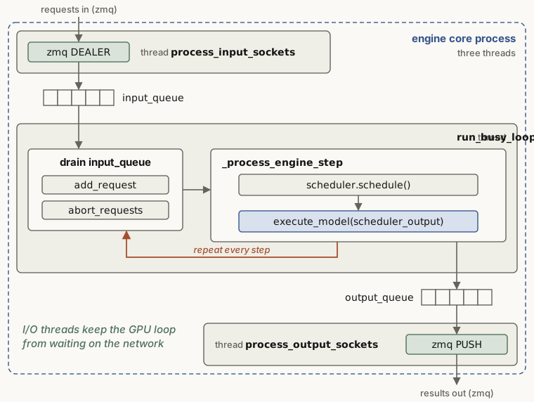
The source article describes the vLLM engine as three modules: the scheduler, KV cache management and the engine core. Figure 35 shows how they work together in one loop.
- Scheduler
- The scheduler looks at the system resources (the token budget and the KV blocks) and at the state of the requests. At each step, it decides which tokens of which requests to compute.
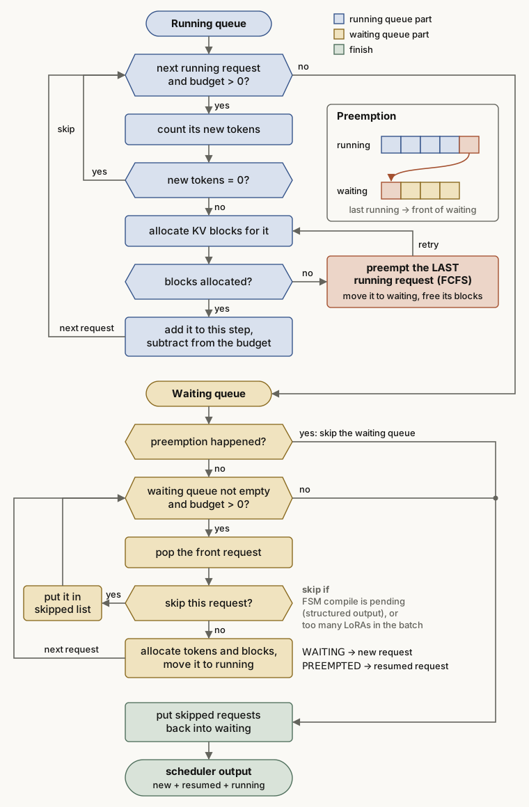
A large flowchart in the source article, in Chinese, shows how the scheduler builds one step. In text, the steps are:
- The scheduler starts with the running queue. It goes through the running requests from the front while the token budget is above 0. For each request, it counts the new tokens to compute in this step. If the count is 0, it skips the request.
- It asks the KV manager for KV blocks. If there are not enough blocks, it preempts the last request in the running list. (This is the default FCFS policy. The priority policy preempts the request with the lowest priority.) It moves that request back to the waiting queue, frees its blocks, and tries again.
- When the blocks are available, it adds the request to the list for this step. It subtracts the tokens of the request from the budget and goes to the next request.
- Next comes the waiting queue. If a preemption just happened, resources are short, so the scheduler skips the waiting queue for this step.
- Otherwise, the scheduler takes requests from the front of the waiting queue. Some requests must wait. For example, the FSM for structured output is not compiled yet, or the batch already has the maximum number of LoRA adapters. These requests go to a skipped list. The scheduler gives the other requests tokens and blocks and moves them to running. A request in the state WAITING counts as new, and a request in the state PREEMPTED counts as resumed.
- At the end, the scheduler puts the skipped requests back into the waiting queue. It then builds the scheduler output from the new requests and the existing ones (resumed and running).
- KV cache management
- Built on PagedAttention. It has a logical layer (the blocks that a request sees) and a physical layer (the real blocks in GPU memory). This is similar to virtual memory management in an operating system.
- Engine core (execution unit)
- Runs the work of one step that the scheduler gives it. This includes the KV transfer and the model execution.
Software and hardware basics
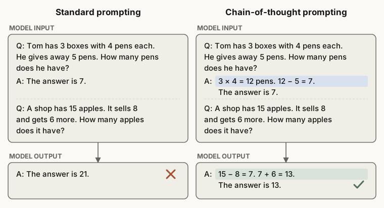
- CoT (chain of thought)
- A prompting method that makes the model show its reasoning steps before the answer. It also matters for inference systems, because it adds many output tokens and so puts more load on decode.
- FCFS (first-come, first-served)
- A scheduling policy that serves the earliest request first. It is the default
schedule_policyin SGLang. - GPTQ
- A one-shot weight quantization method for GPT-style models, with no retraining. It uses approximate second-order information (the Hessian) to correct the quantization error.
- AWQ (activation-aware weight quantization)
- A quantization method that looks at the activation distribution and protects the important weight channels. Before quantization, it multiplies each input channel of the weights by its own scale, which it picks from activation statistics. It then quantizes the weights in groups, often of 128 weights.
- Llama-2-7b-hf
- A naming rule: a Llama 2 model with 7 billion parameters, stored in the Hugging Face format.
- Round robin
- Each task runs for a fixed time slice (for example 10 ms) in turn. If A, B and C arrive in that order, each runs for 10 ms in turn: A, B, C, then A again. Every task gets the same share, so the policy is fair, and no task starves (waits a long time without a turn).
- EOS (end of sequence)
- A special token that marks the end of a sequence. When the model generates EOS, the output stops. EOS is the exit condition of the decode loop in Figure 1.
- logprobs (log probabilities)
- The engine works with ln(p) instead of the probability p. A product of many probabilities quickly comes close to 0 and falls below the range of floating-point numbers (underflow). Logarithms change the product into a sum, so this problem does not occur.
Worked example: why logs
Take the example of the source article, 0.9²⁰⁰. ln(0.9) ≈ −0.105, so after 200 multiplications the log value is about −21.1. This means that 0.9²⁰⁰ ≈ 7 × 10⁻¹⁰. FP32 can still hold this value. But some token probabilities are near 0.01, and a sequence can be thousands of tokens long. Then the product easily drops below the FP32 minimum (about 10⁻³⁸, or about 10⁻⁴⁵ with subnormal numbers). In log space, the same result stays an ordinary number such as −21.1. Beam search also computes its cumulative probabilities as sums of logprobs.
- Reasoning parser
- Separates the output of a reasoning model into the thinking part (for example, the text inside think tags) and the final answer.
- Stream reasoning (streaming output)
- The system sends the results one by one as it generates them. Non-streaming output is the opposite: the system returns everything at once when it is done. With streaming, the user feels TTFT and ITL more than E2EL.
- Structured output
- A feature that makes the output follow a structure, such as a JSON format. Guided decoding (above) implements it. The source article says that the “input” follows the structure, but the constraint applies to the output.
The source article gives an example that applies guided decoding with an SQL grammar. Here it is as code instead of an image.
# Guided decoding with a grammar
simplified_sql_grammar = """
    ?start: select_statement
    ?select_statement: "SELECT " column_list " FROM " table_name
    ?column_list: column_name ("," column_name)*
    ?table_name: identifier
    ?column_name: identifier
    ?identifier: /[a-zA-Z_][a-zA-Z0-9_]*/
"""
guided_decoding_params = GuidedDecodingParams(grammar=simplified_sql_grammar)
The first rule, start, says that the full output must be one SELECT statement. The rule select_statement forces the order “SELECT columns FROM table”. The rule column_list allows several column names with commas between them. The rule identifier uses a regular expression for the name rule: the first character is a letter or an underscore. The last line passes this grammar to GuidedDecodingParams in vLLM. At each step, the engine then sets the probability of every token that the grammar does not allow to 0. Newer vLLM versions removed the guided_* API in v0.12.0. There, the same grammar goes into StructuredOutputsParams(grammar=...).
- RPC (remote procedure call)
- A protocol that lets a program call a function on another computer across the network, as if it were a local function. You do not need to know the network details below it.
- Prometheus
- An open-source monitoring and alerting system, built on a time-series database. Inference servers often use it to collect metrics such as TTFT and throughput.
- ORCA (Open Request Cost Aggregation)
- A standard for how backend servers report their real-time load metrics. A load balancer in front of them, such as an Envoy proxy, reads these reports and spreads the traffic better. The source article names Envoy as an example of a server that reports its load. In ORCA, Envoy is usually the load balancer that reads the reports.
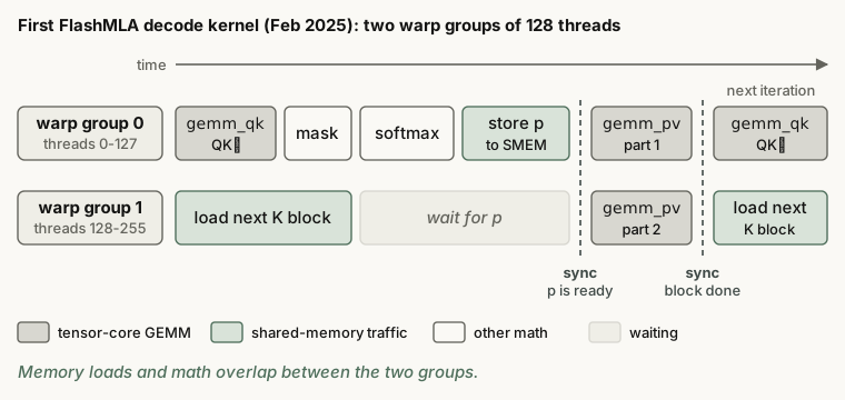
- FlashMLA (multi-head latent attention)
- A library of attention kernels from DeepSeek. It started in February 2025 as an MLA decode kernel for Hopper GPUs. Later releases added prefill and sparse attention kernels.
Python libraries common in inference
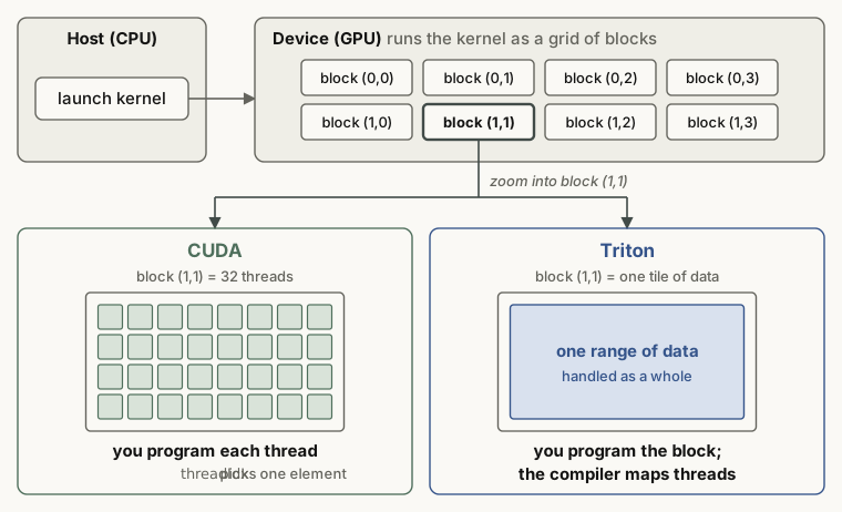
- triton
- A language and compiler for writing GPU kernels in Python at the block level. Older versions included a few ready-made kernels (
triton.ops). Triton 3.2 removed them, and kernels such astriton_kernelsnow come as a separate package.
- ray
- A distributed execution library with flexible resource scheduling. It was first designed for reinforcement learning. In inference, it combines the GPUs of several machines for parallel execution.
- lmcache
- A library that stores and transfers KV cache. Its focus is a lower TTFT through reuse.
- nixl (NVIDIA Inference Xfer Library)
- The data transfer library of NVIDIA for inference. In Dynamo (Figure 31), it moves the KV cache between prefill and decode.
- mooncake
- A library for distributed KV cache storage and transfer. Its TransferEngine is a common choice for cache transfer.
- pytorch
- A general-purpose deep learning framework.
- punica
- A library for multi-LoRA serving. Its SGMV kernel batches requests for many different LoRA adapters on one shared copy of the base model. The project is now archived.
- asyncio
- The standard Python library for concurrent code on a single thread, with an event loop. While one task waits for a network request or for file I/O, the loop switches to another task. Inference servers use it for asynchronous work on the CPU side.
async def main():
    outputs = await llm.async_generate(prompts, sampling_params)
    for prompt, output in zip(prompts, outputs):
        print(f"\nPrompt: {prompt}")
        print(f"Generated text: {output['text']}")
This code comes from an image in the source article. async def defines a coroutine. While await llm.async_generate(...) waits for the generation to finish, the event loop can serve other requests. When the results arrive, the code prints each prompt with its generated text.
- uvloop
- A faster replacement for the asyncio event loop.
- tqdm
- A library that makes progress bars easy. The name comes from the Arabic word “taqaddum” (progress).
- zmq (ZeroMQ)
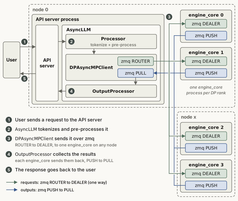
- A high-performance messaging library for distributed and concurrent applications. The vLLM API server and EngineCore use it to talk to each other (Figures 30, 35 and 38).
- fastapi
- A web framework that people often use to build API servers. Its APIRouter groups routes, so the code is easier to read and maintain.
Summary
Material that goes deeper into PagedAttention, PD disaggregation, speculative decoding, FlashAttention and MoE parallelism uses the abbreviations in this post without explanation. When you meet one, first find where it attaches on the map in Figure 1. Then ask which bottleneck it serves: prefill (compute) or decode (memory).
The source article ends with the same kind of advice. When you first learn a concept, search results and LLM answers can be wrong. If two sources disagree, check the original paper and the official documentation first. The different definitions of ITL and TPOT between tools are a good example.
A quick self-check. After this post, you should be able to:
- explain with Figure 2 why prefill is compute-bound and decode is memory-bound;
- say in one sentence which waste each of continuous batching, PagedAttention, APC, chunked prefill and PD disaggregation removes;
- mark TTFT, ITL, TBT, TPOT and E2EL on a time axis and compute them from given numbers;
- apply temperature, top-k, top-p and min-p to one distribution by hand and find the tokens that remain;
- say what DP, TP, PP, SP and EP each split, and what EP = DP × TP means.
Sources
- kaiyuan, 大模型推理核心概念与术语总结 (Zhihu), the source article of this post. Code and notebooks: CalvinXKY/InfraTech.
- Kwon et al., Efficient Memory Management for Large Language Model Serving with PagedAttention, SOSP 2023.
- Zheng et al., SGLang: Efficient Execution of Structured Language Model Programs, NeurIPS 2024.
- Agrawal et al., SARATHI: Efficient LLM Inference by Piggybacking Decodes with Chunked Prefills, 2023.
- Leviathan et al., Fast Inference from Transformers via Speculative Decoding, ICML 2023.
- Dao et al., FlashAttention, 2022, and Dao, FlashAttention-2, 2023.
- Dao et al., Flash-Decoding for long-context inference, 2023.
- FlashInfer team, Accelerating Self-Attentions for LLM Serving with FlashInfer, 2024.
- Wei et al., Chain-of-Thought Prompting Elicits Reasoning in Large Language Models, 2022.
- Frantar et al., GPTQ, 2022, and Lin et al., AWQ, 2023.
- Chen et al., Punica: Multi-Tenant LoRA Serving, 2023.
- The AIBrix team, AIBrix, 2025, and NVIDIA Dynamo.